Simulations of Photo-Induced Properties using LITESOPH
Photophysical and photochemical processes are initiated by the absorption of light by the molecules. After light irradiation molecules get promoted to the electronic excited state, where molecules can undergo a reaction on the same PES or they can deactivate to a ground electronic state via radiative channels like fluorescence and phosphorescence or nonradiative channels like internal conversion ( IC ), and intersystem crossing (ISC). To understand the photophysics and photochemistry of a system, we have to first compute an Absorption Spectrum to get an idea about the optically accessible bright and inaccessible dark states respectively. Then the state of interest can be targeted to understand the photodynamics in the excited state.
Absorption Spectrum
The absorption spectrum provides information about the energies of the electronic excited state and their transition probabilities. The absorption spectrum can be calculated using different theories like TDDFT, CASPT2, CCSD, and ADC (2) [1]. Among all methods, TDDFT offers a good compromise between accuracy and computational cost for a large system [2] [3] [4] [5] [6] . Thus TDDFT is widely used to compute the absorption spectrum. Both linear response (LR)-TDDFT and real-time (RT)-TDDFT can be used to calculate spectrum in frequency and time domain respectively. LITESOPH uses RT-TDDFT approach to compute photoabsorption given its relatively low computational expense for large systems as well as the capability to be given beyond linear response.
Kohn-Sham Decomposition (KSD)
Time-dependent density functional theory (TDDFT) built on top of Kohn-Sham (KS) density functional theory (DFT) is a powerful tool in computational physics and chemistry for accessing the light-matter interaction. Starting from the seminal work on jellium nanoparticles, TDDFT has become an important tool for modeling plasmonic response from a quantum mechanical perspective and has proven to be useful for calculating the response of individual nanoparticles and their compounds as well as other plasmonic materials. Additionally, a number of models and concepts have been developed for quantifying and understanding plasmonic character within the TDDFT approach. TDDFT in the linear-response regime is often formulated in frequency space in terms of the Casida matrix expressed in the Kohn-Sham electron-hole space. The Casida approach directly enables a decomposition of the electronic excitations into the underlying KS electron-hole transitions, which easily provides quantum-mechanical understanding of the plasmonic response. By contrast, real-time TDDFT (RT-TDDFT) (an alternative but computationally efficient approach with favorable scaling with respect to system size and is also applicable to the nonlinear regime) results are often limited to absorption spectra or the analysis of the induced densities or fields. However, recently, Rossi et al. have developed KS decomposition ( KSD ) tool based on the RT-TDDFT code that is available in the free GPAW code. The underlying RT-TDDFT code uses the linear combination of atomic orbitals ( LCAO ) method and enable calculations involving hundreds of noble metal atoms.
In order to analyze the response in terms of the KSD, the decomposition is presented as a transition contribution map ( TCM ), which is an especially useful representation for plasmonic systems in which resonances are typically superpositions of many electron-hole excitations. The TCM represents the KSD weight at a fixed energy of excitation in the two-dimensional plane spanned by the energy axes for occupied and unoccupied states. For more details, refer to [7].
More specifically, the 2D plot is defined by
where indices \(i\) and \(a\) correspond to the occupied and unoccupied states, respectively. The function \(g_{ia}\) is a 2D broadening function for the discrete KS \(i \rightarrow a\) transition contributions. By employing the 2D Gaussian function, it is written as
where \(\sigma\) is the broadening parameter, which is generally taken to be the same as used for the spectral broadening.
The weight \(w_{ia}(\omega)\) in Eq. \(\ref{eq:1}\) is obtained from the absorption decomposition normalized by the total absorption, i.e.
We note here is that the above equation is given particularly for the x-polarized light. However, the same thing can also be evaluated for y or z-polarized light.
The KS decomposition of the absorption spectrum in Eq. \(\ref{eq:3}\) is defined as
where the dipole matrix element is obtained as
where \(\psi_j^{(0)}\) corresponds to the KS wave function for \(j = i,a\).
The linear response of the real part of the KS density matrix in the electron-hole space is written as
where \(K_x\) is the laser strength and \(\rho_{ia}(0^{0-})\) is the initial density matrix before the \(\delta\)-pulse perturbation, and the superscript \(x\) indicates the direction of the perturbation.
Transition contribution map for the photoabsorption decomposition of Au55 metallic nanoparticle at 3.02 eV resonance energy calculated using LCAO TDDFT approach in GPAW code is shown in Fig.1.
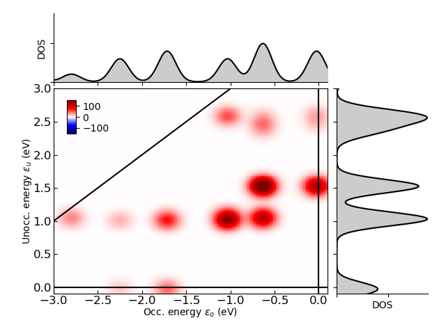
Fig.1: Transition contribution map for the photoabsorption decomposition of Ag55 metallic nanoparticle at 4.0 eV resonance energy calculated using LCAO TDDFT approach in GPAW code. The KS eigenvalues are given with respect to the Fermi level. The constant transition energy line \(\varepsilon_u - \varepsilon_o = \omega\) is the analysis energy (solid line). Red and blue colors indicate positive and negative values of the photoabsorption, respectively. The density of states (DOS) are also shown.
Molecular Orbital (MO) Population
The Kohn-Sham (KS) orbital can be expanded using gaussian basis function \(\phi_\mu\) as:
Density matrix can be obtained from the products of time-dependent coefficient:
Time dependent orbital population computed by projecting the density matrix on to the ground state orbitals:
LASER Simulation
Once we have the photoabsorption spectrum of any system, we get an information about the excitation frequencies present in the system. Using any frequency of excitation, we can hit the system with a laser and study the time dynamics of any physical observable of our interest.
The Gaussian light pulse is defined as
that induces a real time dynamics in the system. The pulse frequency \(\omega_0\) is tuned to the frequency of excitation of interest, the pulse duration is determined by \(\sigma\), and the pulse is centered at \(t_0\). The pulse strength \(\varepsilon_0\) is generally kept weak, to ensure that the system is in the linear response regime. In the frequency space, the pulse should be wide enough to cover the whole frequency of excitation.
The determination of the pulse width and its center is crucial for the light-matter interaction. However, these quantities can be evaluated from the envelope function in Eq. \(\ref{eq:laser_pulse}\), which is defined as
The Gaussian envelope in time will also yield the Gaussian envelope in frequency (Gaussians are eigenfunctions of a Fourier transform), with width equal to the inverse of the width in time. The full width at half maximum ( FWHM ) of Gaussian pulse is given as
The center of the pulse is obtained as
LASER Masking approach to study energy transfer using RT-TDDFT approach
Energy transfer is one of the most fundamental processes on the molecular scale, governing light harvesting in biological systems and energy conversion in electronic devices such as organic solar cells or light-emitting diodes. The design principles of natural light-harvesting complexes have found considerable interest, as scientists believe that the principles realized in nature can be mimicked in the design of artificial organic devices. One standard method to interpret experimental data of excitation energy transfer between a donor (D) and an acceptor (A) molecule separated by the distance R is the so-called Forster resonance energy transfer ( FRET ) theory. \(Forster\) theory describes ¨ the nonradiative energy transfer mediated by a (quantum-mechanical) coupling between the transition dipoles of the donor and acceptor molecules. One of the central assumptions in FRET is that the coupling between D and A can be described by a (point)-dipole-dipole interaction, falling as 1/R3. Furthermore, FRET theory is formulated for the weak coupling regime (i.e., the isolated D and A excited states do not change significantly on coupling).
The energy transfer rate is written as
where \(\mathbf J(\varepsilon)\) is the spectral overlap between the normalized donor emission and acceptor absorption spectra.
The factor V in Eq. \(\ref{Eq:K^ET}\) is the electronic coupling matrix element which is obtained using Davydov splitting. In the case two same molecules, the Davydov splitting \(\Delta\Omega\) equals the energy splitting \(\Delta E\) of the (nearly) degenerate excitation energies of the monomers in the supermolecule.
There is however, an another alternative way of evaluating the required information by observing the \(D\) and \(A\) dipole moments separately. It significantly reduces the computational cost. We note that the Davydov splitting and consequently also the coupling matrix element \(V\) manifests itself as a frequency \(\omega_{beat}\) in the time-dependent \(D\) (and \(A\)) dipole moment. This frequency can be extracted as a beat frequency \(\omega_{beat}\) of an oscillation between \(D\) and \(A\).