RT-TDDFT
The RT-TDDFT calculations can be performed starting with external perturbations, such as, Delta pulse and laser pulse. For the input parameters of delta pulse, see Delta kick Inputs. For the input parameters of laser pulse, see Laser Design tools.
Delta kick Inputs
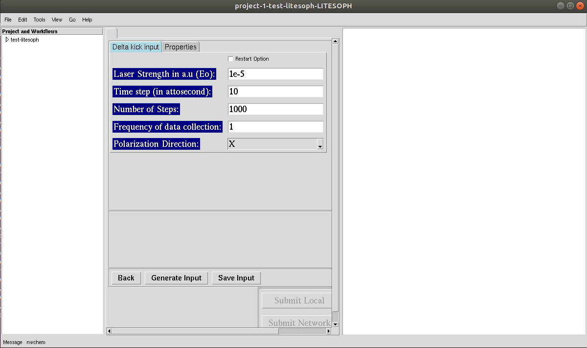
1. Laser Strength in a.u (E0): Strength of the delta kick electric field to be applied. This excites all the electronic degrees of freedom at the beginning.
2. Time steps (in attosecond): Time steps for the dynamics of the Kohn-Sham equations.
3. Number of Steps: Total number of steps to be run for the dynamics. Total time is (Number of Steps*time steps)
4. Frequency of data collection: Number of times the data will be printed. Default alue \(1\) indicates that data will be collected at each time steps.
5. Polarisation Direction: Polarization direction of the applied external electric field.
Click on Restart Option, if applicable. Posible options include: increasing number of simulation steps.
Note
All the input parameters will be collected to generate input if Restart Option is chosen. Make sure to change only the relevant parameters such as: Number of Steps. Any modification of External Fields should be avoided.
Laser Design tools
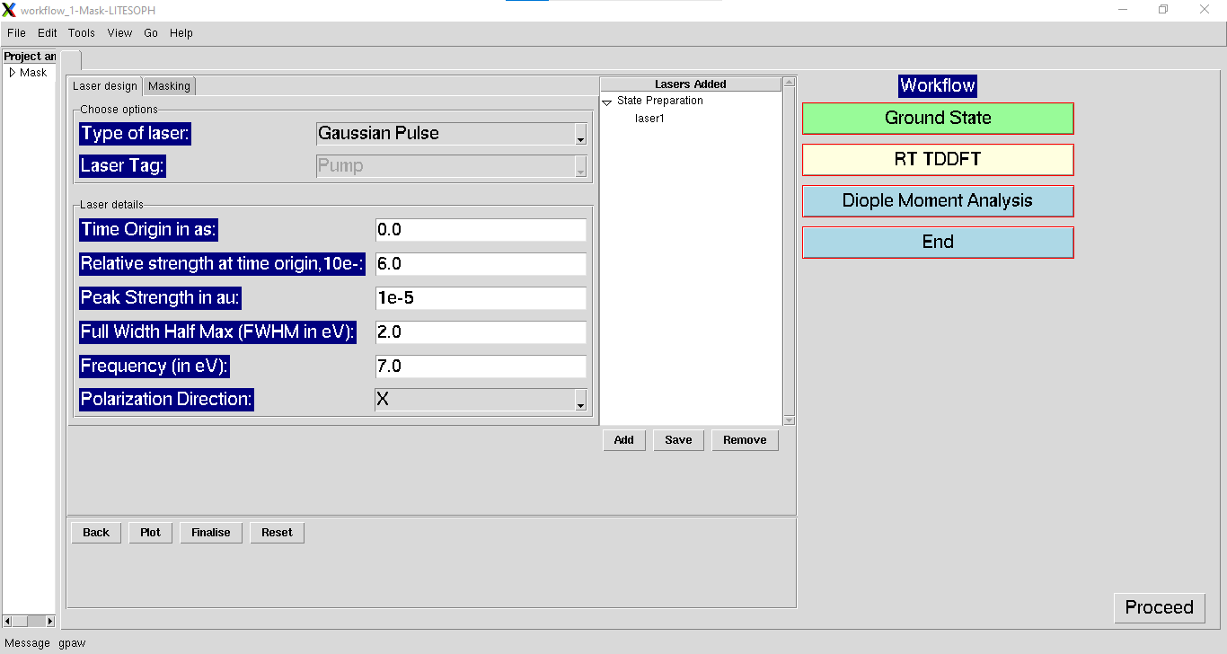
Laser design
1. Type of Laser: (default:Gaussian) Available options are Gaussian pulse and Delta pulse.
2. Laser Tag: (default:Pump) Applicable only in the case of Pump-Probe analysis. Choose either pump or probe for laser design.
For the parameters of Delta kick, refer to Delta kick Inputs.
For the parameters of Gaussian pulse, see below.
1. Time Origin (as): (default:0) Laser delay time from initialization of simulation in atto-seconds.
2. Relative strength at time origin, 10e-: (default:6) Negative log of relative electric field strength at the starting time of the laser.
3. Peak Strength (au): (default:10e-5) Intensity of laser in au.
4. Full Width Half Max (eV): (default:1) FWHM of the Gaussian pulse.
5. Frequency (eV): (default:1) Frequency of the Gaussian pulse.
6. Polarization Direction: (default:X) Polarization Direction of the applied electric field.
Add and Save the lasers and view the laser using Plot.
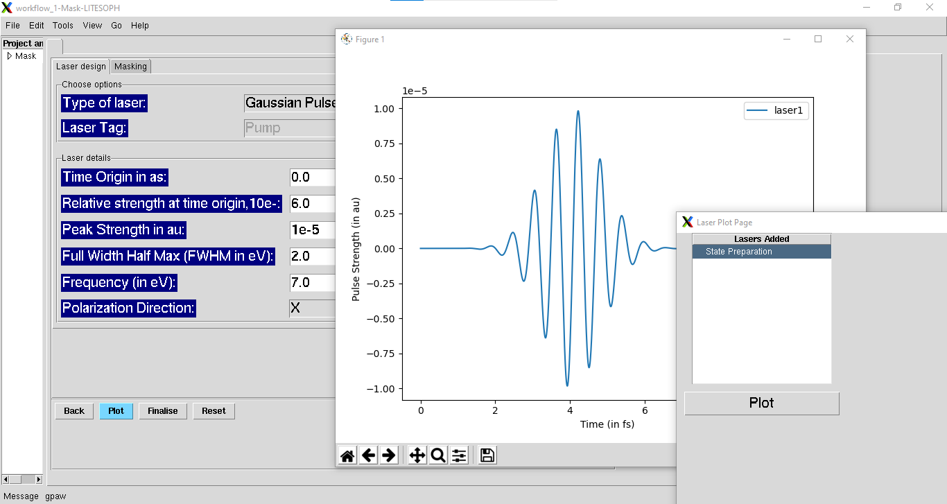
Finalise the laser which will be used for further simulations.
Masking
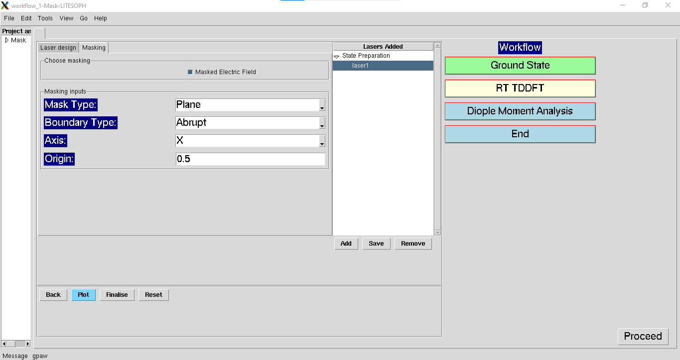
Select the added lasers for which masking is to be applied. Under masking, check the Masked Electric Field. Use the following input parameters for masking. This is optionally used to select a region to illuminate for the chosen laser.
1. Mask Type: (default:Plane) Types of mask defined as boundary to separate the masked and illuminated regions. Available options are :Plane and Sphere.
Plane: refers to the use of a dividing plane to define the mask
Sphere: refers to the use of a spherical region to illuminate
2. Boundary Type: (default:Abrupt) Smearing type at the mask boundary. Available options are Abrupt and Smooth.
Abrupt: refers to an abrupt division of cell i.e. using a Heaviside function
Smooth: refers to the boundary region being defined through an error function
3. RSig: (default:0.1) Applicable for Boundary Type: Smooth. Refers to sigma (in Angstroms) of the error function to be used
Mask Specific Parameters
4. Axis: (default:X) Applicable for Mask Type: Plane. Direction along which the boundary is placed.
- 5. Origin:
(default:0.5) Applicable for Mask Type: Plane. The location of the dividing plane (in cell parameter units). Only for coordinate < origin, the region is illuminated.
(default:(0.5, 0.5, 0.5)) Applicable for Mask Type: Sphere. Coordinates (in cell parameter units) of the centre of the Sphere used
6. Radius: (default:0.5) Applicable for Mask Type: Sphere. Radius (in Angstroms) of the spherical region to be illuminated
Save the masking details after including the above parameters.
Properties
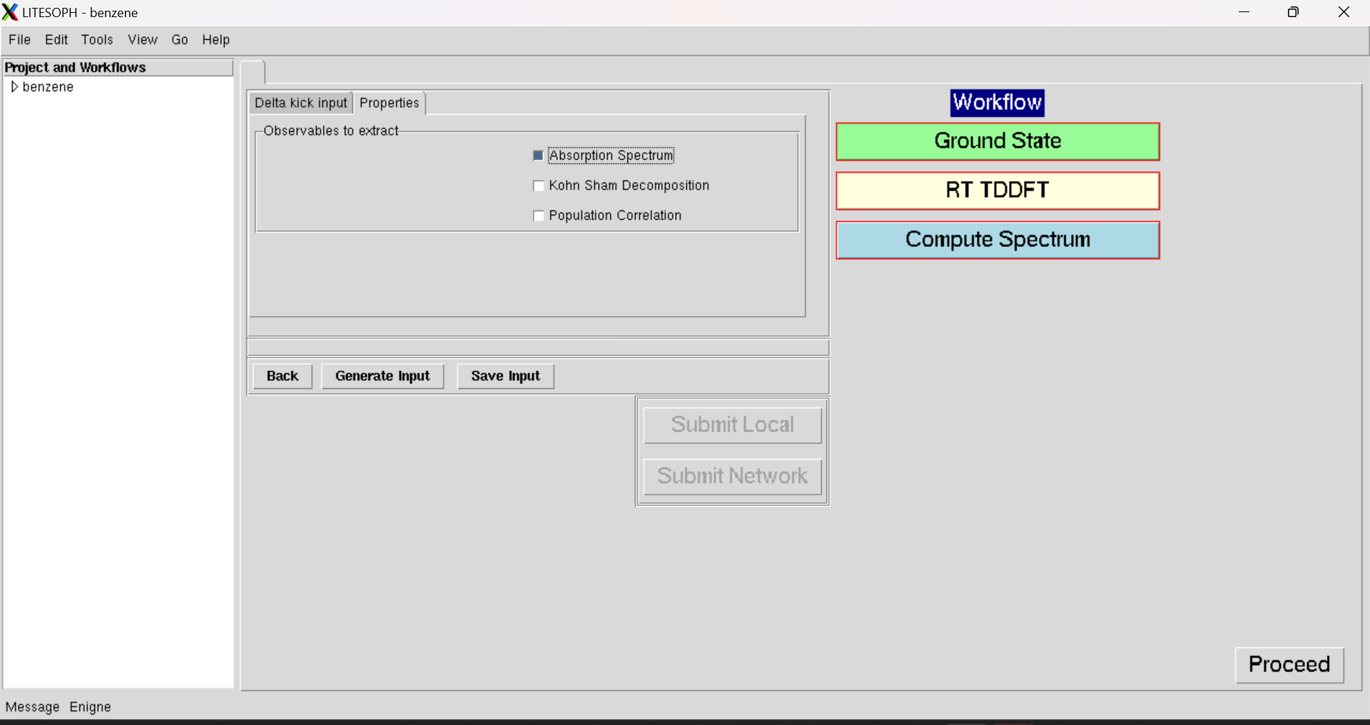
1. Observables to extract: Choose the operation to be performed.
For Spectrum Calculation choose Absorption Spectrum.
For KSD calculation choose Absorption Spectrum and Kohn Sham Decomposition.
For MO population calculation choose Absorption Spectrum, Kohn Sham Decomposition and Population Correlation.